Giving the robot an imperfect estimate
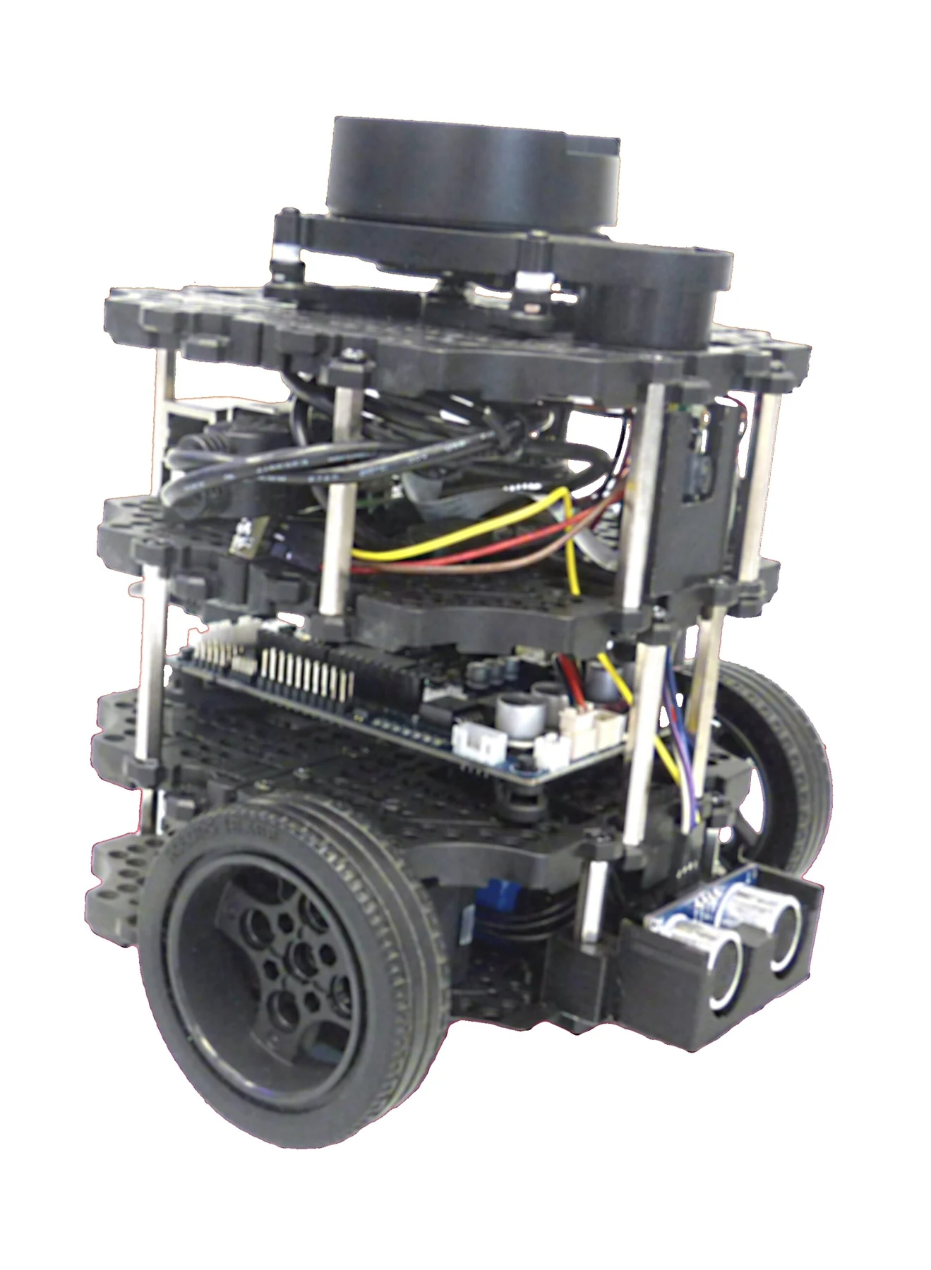
I built a differential-drive simulator with A* path planning, heading control, wheel encoders, an IMU, and extended Kalman filter localization. The question was what the robot should do when its estimate of its own position becomes unreliable.
I injected encoder noise, IMU drift, yaw bias, and wheel slip. This made it possible to inspect failures that would be hidden by perfect simulated sensing.
Connecting wheel motion to the estimate
For an ideal differential drive with equal wheel radii, forward speed and heading rate are:
r is wheel radius, b is the distance between the wheels, and ωᴿ and ωᴸ are their angular velocities. This differential-drive model is a starting point; wheel slip means measured wheel rotation does not always translate into the motion predicted by the ideal model.
The EKF tracks uncertainty as well as state. Its prediction step propagates the covariance:
P is the state covariance, F is the local linearization of the motion model, and Q represents process uncertainty. The measurement update then corrects the prediction using sensor information. MathWorks’ EKF explanation gives the underlying prediction and correction structure.
Deciding when to slow down or recover
I implemented confidence-aware speed and recovery logic so the robot could respond when localization became unreliable. Planning a route, following it, and deciding whether to trust the current state estimate all belong in the navigation loop.
Looking beyond arrival
I evaluated the stack through Monte Carlo trials, tracking collisions, localization error, recovery events, success, and time to goal. Reaching the target alone would not explain whether the route was safe or how often recovery was needed.
This was a simulation project. The results and workflow concern the simulated robot and disturbances, rather than field validation on physical hardware.