A joint whose stiffness can change
I’m studying how a tensegrity joint responds when its geometry and internal loading change. The longer-term interest is a wearable or exoskeleton joint, where the same mechanism may need to give way in one situation and resist motion in another.
My current work is a MATLAB study of member forces, force output, and joint stiffness. I vary geometry, external loading, and internal force to understand which changes have the largest effect, then use those comparisons to narrow the design.
Following the member forces
A useful starting point is equilibrium. With a consistent force convention, the member forces and external load must balance:
A(q) describes how the members are arranged at configuration q. The vector t contains their axial forces, and fₑₓₜ contains the external loads. The geometry matters because it determines how an individual member’s force contributes to the overall balance. Cable forces also need to remain consistent with cables carrying tension.
For rotational response, local joint stiffness can be described by:
Here, θ is joint angle and τ is the resisting torque along the response being examined. I’m interested in how that slope changes across configurations and loading conditions. A single stiffness value does not describe the whole motion.
Connecting the analysis to the mechanism
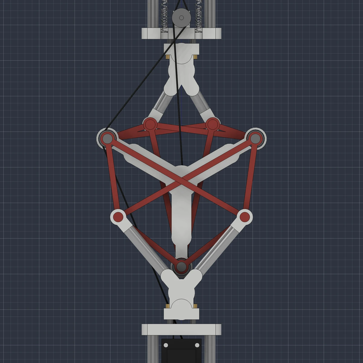
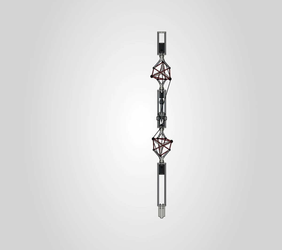
The CAD views help me inspect the geometry and how the joint fits into a leg assembly. They are a paper-based mechanism reconstruction used for study, drawing on Mortensen and colleagues’ tensegrity leg design.
The next step is to carry a small set of useful configurations into a physical prototype. The modeling is still ongoing; the wearable application is a direction for later development.