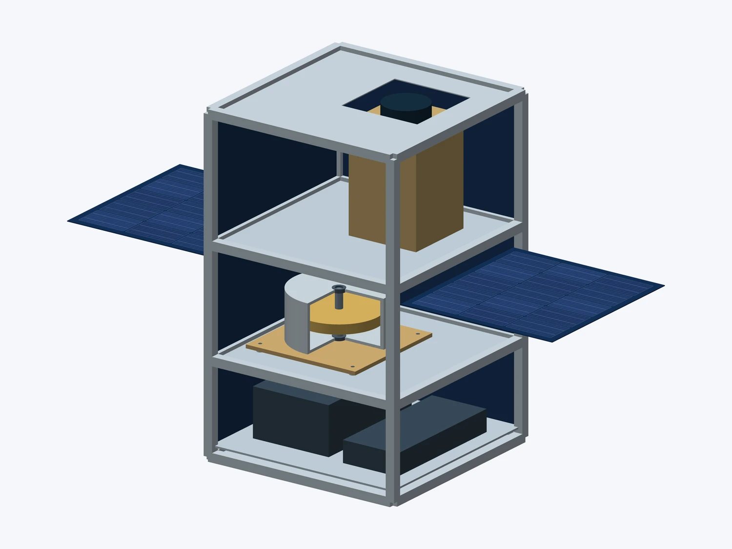
Looking at the camera interface
I modeled how reaction-wheel microvibration travels from the wheel mount through a satellite panel to the camera interface. I wanted to follow the disturbance to the payload location, rather than stop at identifying where the panel resonates.
The study uses modal and harmonic FEM. Modal analysis identifies the structure’s modes and natural frequencies. Harmonic analysis then examines its response to periodic excitation.
The harmonic model
For a linear structural model, the frequency-domain equation can be written as:
M, C, and K are the mass, damping, and stiffness matrices. The complex displacement amplitude q̂ is the response to the force amplitude f̂ at angular frequency ω. Evaluating the camera interface connects this model to the location of interest.
Wheel speed also needs to be related carefully to excitation frequency. For the fundamental rotational frequency:
n is rotational speed in rpm and fᵣₒₜ is in hertz. Other excitation components can occur at harmonics of that frequency; the relationship alone does not define every disturbance produced by a wheel.
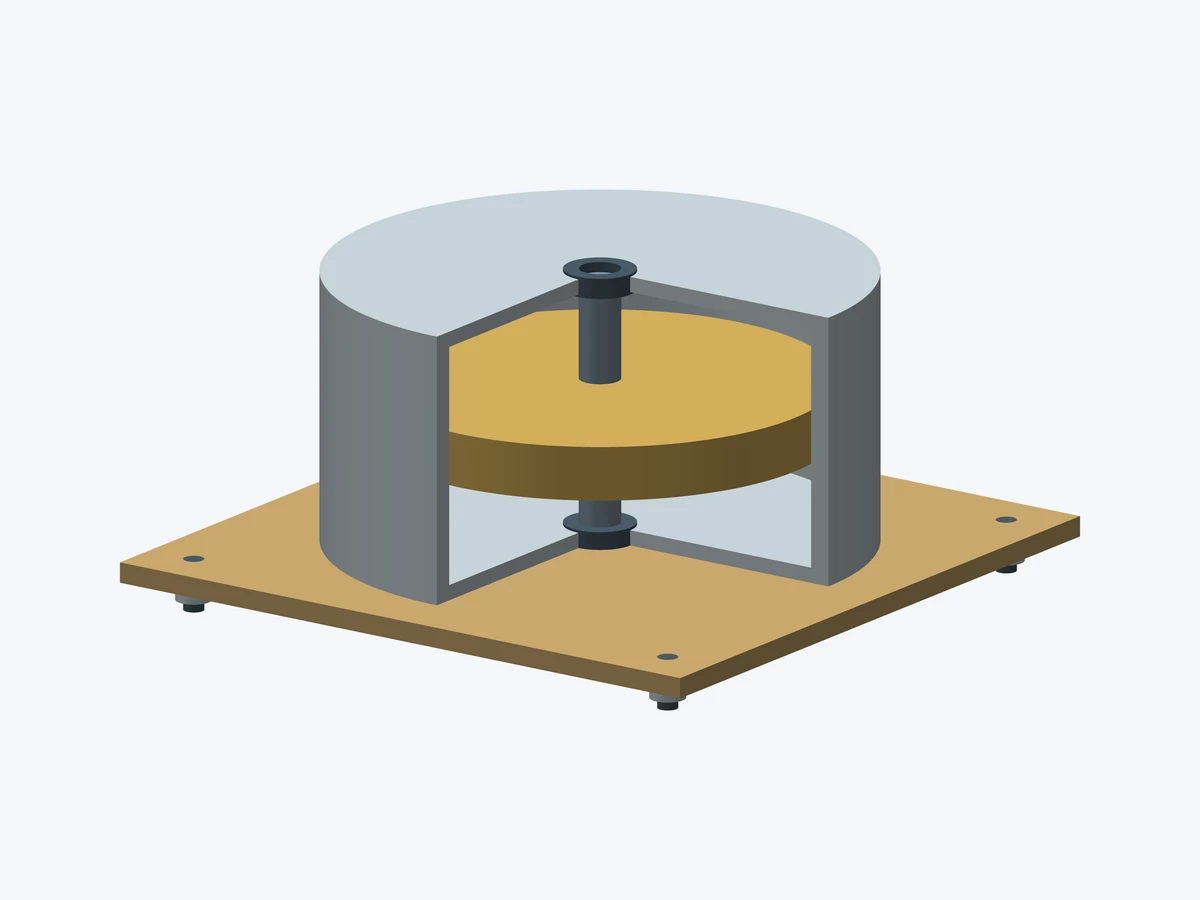
Checking the response peak
The model showed a strong camera response near 5,800 rpm. I refined the mesh to test whether the peak depended too strongly on the discretization. The amplitude changed by 0.33% between the compared meshes.
That number is a mesh-sensitivity result. It does not establish experimental accuracy, but it helps assess whether the peak is stable under the particular refinement being compared.
Exploring a faster predictor
I structured a 24-design parameter sweep and a held-out regression check to explore when a surrogate model could follow the FEM response. Resonance is an important place to examine its errors: a smooth-looking prediction could still miss a narrow peak.
The completed work is a simulation study and regression-evaluation workflow. Experimental validation remains separate.